

精细研究大气边界层特性常用的风工程方法主要有现场实测、风洞实验和数值模拟等3类.与现场实测和风洞实验相比,数值模拟方法不受探测技术、设备性能、地理因素等客观因素限制,成为使用更多的研究手段.Fluent等经典软件未考虑地表能量平衡计算、云微物理参数化等气象模式,因此在真实大气应用中存在一定缺陷;此外,由于运算能力和时间的限制,Fluent等经典软件不适合较大范围的风场模拟,而数值天气预报(Weather Research and Forecasting,WRF)系统可以弥补这些缺陷.WRF模式具有参数多、方案新、精度高、易嵌套等特点和优点,可用于预测、重现大气边界层风场特性.文献[5]中利用WRF模式数值模拟兰州河谷盆地区域,获得的风场和温度场模拟结果与观测基本一致,为缓解城市热岛效应提供了参考依据.文献[6]中采用WRF模式对台风“鹦鹉”进行高时空分辨率模拟,通过分析台风模拟路径、气压分布、风速模式等风场特性,发现WRF模式能有效模拟近地面台风风场,为后续小尺度数值模拟提供真实的入流风场.Yuan等[7]采用WRF模式对真实陆上风电场内的流动特性和功率输出特性展开高分辨的数值模拟,利用风电场的观测数据进行验证,结果表明,WRF模式对于风场的风速、风向和风力机功率的模拟具有较高的精度.WRF模式汇聚了不同学者描述不同物理过程的参数化方案,它们各有特点和使用条件限制,因而会影响数值模拟的稳定性和精度,如空间差分格式方案和次网格模型方案对精细化模拟产生影响.Wicker等[8]对比通量的三阶、四阶、五阶和六阶形式,发现奇数阶算法是更高一阶(偶数阶)算法的线性组合,具有数值耗散性.Janjic等[9]在非线性试验中发现四阶差分格式比原始二阶差分格式对于小尺度能量积累更具有优势.Yamaguchi等[10]研究发现高阶对流方案有利于减少云模式的数值耗散.文献[11]中设计25个试验(水平对流项和垂直对流项分别采用二阶~六阶5种差分格式),开展非线性密度流试验研究,通过分析涡旋产生位置和发展,发现水平五阶差分和垂直三阶差分的组合方案,基本可消除不稳定扰动.大涡模拟(Large-Eddy Simulation, LES)方法通过直接求解大尺度涡,采用次网格模型参数化小尺度涡,有利于精细化模拟近地面风场,Deardoff[12]在1972年将大涡模拟应用于大气边界层的模拟.现有WRF版本集合了LES模块,通过修正WRF-LES模块的次网格模型而较好地呈现近地面风场特性.Moeng[13]在1984年LES中也采用了TKE闭合模式,但该方法所模拟的平均风速在近地面附近不满足相似理论的对数律.Moeng等[14]也在传统的Smagorinsky次网格模型添加修正项,以减小不同计算域间的表面摩擦偏差,改进后的模型较好地重现了热力驱动或风切变引起的边界层湍流特性,提高了大涡模拟的精度.Leith [15]考虑了湍能的逆向串级,提出随机后向散射次网格闭合模式.Mirocha等[16]在WRF-LES中添加非线性回波散射和各向异性(Nonlinear Backscatter and Anisotropy,NBA)模型,与线性模型相比,NBA模型明显降低近地面风速剖面与对数律预期之间的偏差,从瞬时风场图中发现其模拟的涡旋尺寸范围更广,能更好描述高分辨率下地面附近的流动分离.Kirkil等[17]利用WRF模式研究了拉格朗日平均尺度相关模型和动态重构模型,研究结果表明这两种动态次网格应力模型能够很好预测功率谱中惯性区域的产生和范围扩展,实现最好的动态模型的整体缩放,这种效果在地表附近效果更加明显.此外,网格分辨率也影响模拟的精度,Zheng等[18]发现提高网格分辨率对空气污染、降雨降水的预测非常重要.文献[19]中利用WRF-LES模式评估3种水平网格分辨率(120、60、30 m)和3种垂直网格分辨率(20、10、5 m)对对流层的影响,发现水平网格分辨率为30 m时,能在大气边界层范围获得理想的湍流再现,而垂直网格分辨率的提高对模拟结果影响较小.Mirocha等[16]发现网格纵横比(水平网格分辨率/垂直分辨率)为3~4时,平均风速剖面更加接近指数律.
上述研究运用WRF-LES模式模拟大气边界层,多采用均匀网格,尚缺少加密网格和非线性次网格模型、空间差分格式奇偶性对近地面风场精细化模拟影响的深入研究,可能会导致该模型难以准确模拟大气边界层近地风场特性.
本文基于WRF-LES模式,寻找适用于近地面风场精细化模拟的次网格模型方案、空间差分方案和网格设置方法.首先阐明数值模型的控制方程和湍流模型,然后阐述数值模拟方法,包括大气边界层的几何模型、边界条件和计算设置,随后讨论和分析了计算结果,最后进行总结.
1 数值模型
1.1 控制方程
利用WRF-LES模式开展理想大气边界层近地面风场特性的数值模拟,为了定量描述和预报边界层状况,文献[20]中引入可压缩流体的状态方程、连续性方程、动量方程、热力学方程和水分方程.考虑易读性,简化方程表示如下.
状态方程:
连续性方程:
动量方程:
热力学方程:
水分方程:
式中:
将动量方程在空间上进行过滤,只滤去小波脉动,保留大涡脉动,可得:
式中:
1.2 湍流模型
式中:
2 数值模拟方法
2.1 几何模型与计算网格
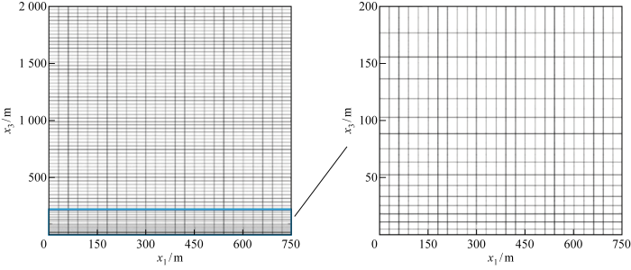
通过WRF-LES模式构建模型,以理想大气边界层为研究对象,研究次网格模型方案、网格分辨率方案和空间差分格式方案对大气边界层近地面风场特性的影响.表1给出理想大气边界层的模拟范围,水平和垂直的网格分辨率和网格数量,以及时间步长.对于次网格模型试验,水平网格分辨率取30 m,垂直网格分辨率取20 m,选用WRF4.3提供的4种次网格模型.对于网格分辨率试验,在一个基本算例(水平网格分辨率30 m,垂直网格分辨率 10 m)的基础上,选用只改变水平网格分辨率的4种试验方案和只改变垂直网格分辨率的5种试验方案.其中,不均匀加密方案的计算域如图1所示,入口风速为15 m/s,计算域长宽为 6 000 m,计算高度为 2 000 m.水平方向上网格分辨率取30 m,网格数为200×200,网格节点均匀分布.垂直方向上采用拉伸网格方案,如图2所示.图中:x1、x3分别为经度坐标和垂直坐标.在离地200 m范围内加密16层,第1层网格高度近似为3.54 m,网格膨胀率为1.1;200 m以上采用间距30 m的均匀网格.垂直网格不均匀加密方法可以在使用少量网格情况下,解决壁面黏性切应力的影响.对于空间差分格式试验,H代表水平对流,V代表垂直对流,例如H5V3表示为水平对流项取五阶差分,垂直对流项取三阶差分.
表1 基于WRF-LES的次网格模型方案、网格分辨率分案和空间差分格式的试验模拟参数
Tab.1
| 试验名称 | 空间差分格式 | 次网格模型 | Δx/m | Δx3/m | 水平网格数量× 垂直网格数量 | 时间步长/s |
|---|---|---|---|---|---|---|
| 次网格模型 | H5V3 | TKE | 30 | 20 | 200×100 | 0.25 |
| H5V3 | SMAG | 30 | 20 | 200×100 | 0.25 | |
| H5V3 | NBA1 | 30 | 20 | 200×100 | 0.25 | |
| H5V3 | NBA2 | 30 | 20 | 200×100 | 0.25 | |
| 网格分辨率 | H5V3 | NBA1 | 15 | 10 | 200×200 | 0.10 |
| H5V3 | NBA1 | 30 | 10 | 200×200 | 0.25 | |
| H5V3 | NBA1 | 60 | 10 | 100×200 | 0.50 | |
| H5V3 | NBA1 | 120 | 10 | 50×200 | 0.50 | |
| H5V3 | NBA1 | 30 | 5 | 200×400 | 0.25 | |
| H5V3 | NBA1 | 30 | 10 | 200×200 | 0.25 | |
| H5V3 | NBA1 | 30 | 20 | 200×100 | 0.25 | |
| H5V3 | NBA1 | 30 | 30 | 200×66 | 0.25 | |
| H5V3 | NBA1 | 30 | 不均匀加密 | 200×77 | 0.25 | |
| 空间差分格式 | H3V3 | NBA1 | 60 | 10 | 100×200 | 0.50 |
| H4V2 | NBA1 | 60 | 10 | 100×200 | 0.50 | |
| H4V4 | NBA1 | 60 | 10 | 100×200 | 0.50 | |
| H5V3 | NBA1 | 60 | 10 | 100×200 | 0.50 | |
| H5V5 | NBA1 | 60 | 10 | 100×200 | 0.50 | |
| H6V4 | NBA1 | 60 | 10 | 100×200 | 0.50 | |
| H6V6 | NBA1 | 60 | 10 | 100×200 | 0.50 |
图1
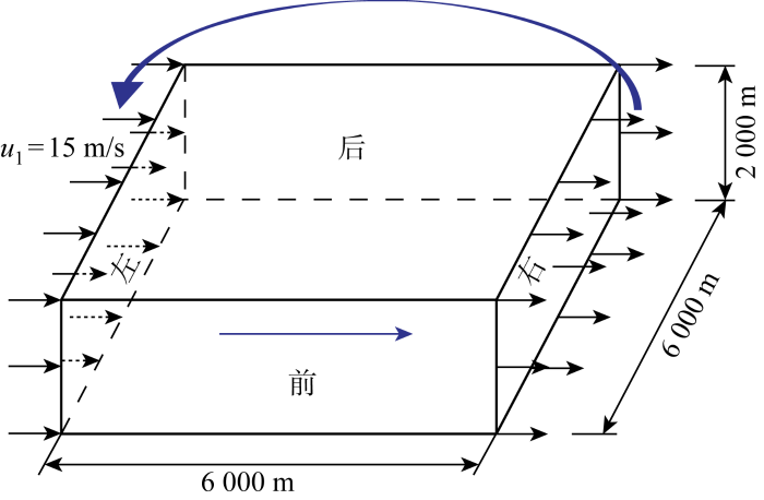
图2
2.2 计算设置
计算域左侧为速度入口,右侧为速度出口,前后左右均为周期性边界条件,顶部边界条件光滑无渗透,表面层方案采用基于Monin-Obukhov相似理论[22]的改进MM5方案,该相似理论与风工程中常用的壁面函数一致,由以下公式确定:
式中:τsurf为地表摩擦力;u*为摩擦速度;ua为z高度处的风速;Cd为摩擦因数;z0为地面粗糙度;κ为von Karman常数,取值0.4;L为Obukhov长度;U为顺风向风速;ψ为大气稳定度的方程[23],在此不赘述.
地面粗糙长度设为0.1 m.时间积分方案采用三阶Runge-Kutta方法.所有其他物理选项均关闭,如微物理过程、积云方案、陆面过程、辐射过程等.计算时间为20 h(次网格模型中的NBA1和NBA2方案除外),每隔1 h存储一次模拟的全流域结果.设立55个监测点,记录每个时间步监测点剖面的风速,最后2 h的监测点数据用于结果统计分析.将最后2 h的统计数据与更长时间计算得到的数据进行对比,发现二者数据较为吻合,验证了时长的独立性.
3 WRF-LES计算方法验证
图3

4 计算结果和分析
4.1 次网格模型对大气边界层模拟结果的影响
图4
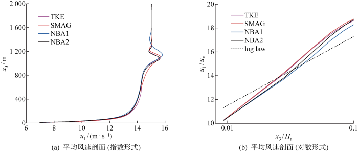
图4
不同的次网格模型方案下平均风速剖面
Fig.4
Mean wind speed profiles of different subfilter-scale stress models
表2 不同的次网格模型方案下平均风速模拟结果与对数律的相对误差
Tab.2
| 次网格 模型 | 不同高度处的平均风速相对误差/% | |||||
|---|---|---|---|---|---|---|
| 9 m | 28 m | 47 m | 65 m | 84 m | 103 m | |
| TKE | -9.23 | 0.60 | 5.79 | 7.91 | 8.24 | 7.80 |
| SMAG | -9.22 | 1.12 | 6.00 | 8.60 | 9.02 | 8.55 |
| NBA1 | -9.36 | -2.61 | 1.41 | 4.56 | 5.74 | 5.88 |
| NBA2 | -9.53 | -1.94 | 3.63 | 6.90 | 8.15 | 8.28 |
图5给出近地面范围内不同次网格模型的水平方向湍流强度I1,可看出湍流强度基本在0.12~0.22波动,而且30~100 m高度内NBA模型的湍流强度明显大于标准TKE模型或SMAG模型,在相同的高度处,不同次网格模型间的相对误差可达到10%,这可能是因为NBA中的非线性成分对来流扰动作用增强,使得湍流强度更大.
图5
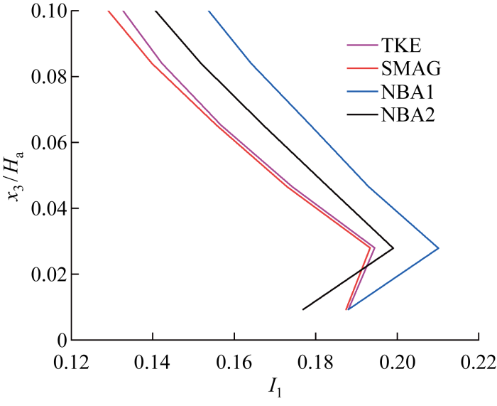
图5
不同的次网格模型方案下湍流强度剖面
Fig.5
Turbulence intensity profiles of different subfilter-scale stress models
取所有监测点的顺风向风速序列,分别做功率谱,空间平均后再拟合处理,具体结果如图6所示.图中:
图6
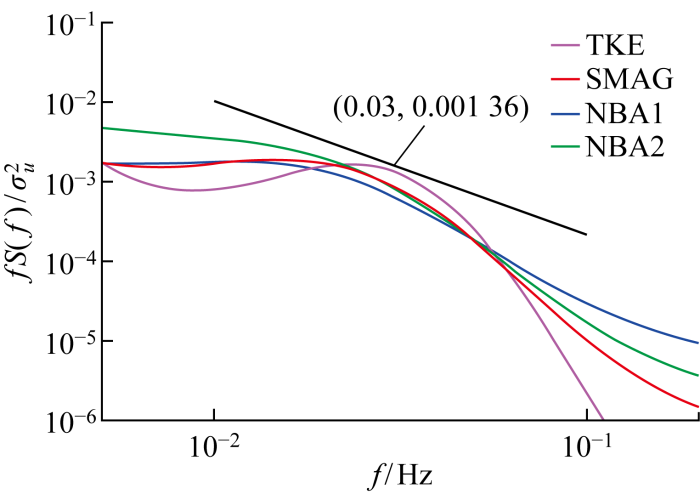
图6
在100 m高度处,不同的次网格模型方案的功率谱
Fig.6
Power spectrum of different subfilter-scale stress models at 100 m above the surface
式中:λe为有效网格分辨率;fe为有效频率.
因此,综合水平风速剖面、湍流强度剖面和有效网格分辨率等方面考虑,确定NBA1模型为次网格模型的最佳选择.
4.2 网格分辨率对大气边界层模拟结果的影响
网格分辨率对数值模拟的影响是一个相对复杂的问题.一方面数值模拟精度依赖于网格分辨率,为提高数值模拟精度要求网格分辨率尽可能高,尤其是在壁面附近;另一方面,受计算条件限制,网格分辨率不能无限增加.因此,讨论如何在节约计算资源下优化网格设计,使得模拟结果真实可靠.
根据表1网格分辨率设计试验,将模拟结果绘制成平均风速剖面如图7所示,统计平均风速的相对误差如表3所示.其中dx代表水平网格分辨率,dz代表垂直网格分辨率,例如dx15dz10表示水平网格分辨率取15 m,垂直网格分辨率取10 m.通过图7(a)、7(b)的对比,发现水平分辨率从30 m加密到15 m,垂直网格分辨率从30 m加密到10 m,平均风速剖面的结果对水平网格改变反而更加敏感,而垂直网格的改变对结果基本无明显影响.文献[6]中也发现类似现象.混合长度可能是造成这种结果的原因之一.本试验中水平和垂直均采用相同的混合长度,当水平网格分辨率提高一倍,混合长度增加
图7
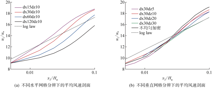
图7
不同水平网格分辨率和垂直网格分辨方案的平均风速剖面
Fig.7
Mean wind speed profiles of different mesh resolution cases
表3 不同水平网格分辨率和垂直网格分辨率方案下平均风速模拟结果与对数律的相对误差
Tab.3
| 试验方案 | 水平网格 尺寸/m | 垂直网格 尺寸/m | 垂直网格 最小尺寸/m | 纵横比 | 不同高度处的平均风速相对误差/% | |
|---|---|---|---|---|---|---|
| 15 m | 45 m | |||||
| dx15dz10 | 15 | 10 | 4.65 | 1.5 | 0.11 | 9.98 |
| dx30dz10 | 30 | 10 | 4.65 | 3 | -8.01 | 3.62 |
| dx60dz10 | 60 | 10 | 4.65 | 6 | -14.51 | -7.53 |
| dx120dz10 | 120 | 10 | 4.65 | 12 | -18.73 | -17.82 |
| dx30dz5 | 30 | 5 | 2.32 | 6 | -9.63 | 4.65 |
| dx30dz10 | 30 | 10 | 4.65 | 3 | -8.01 | 3.62 |
| dx30dz20 | 30 | 20 | 9.31 | 1.5 | -19.33 | 2.25 |
| dx30dz30 | 30 | 30 | 14.11 | 1 | -12.91 | -1.14 |
| 不均匀加密 | 30 | — | 3.54 | — | -5.76 | 9.64 |
图8给出不同网格分辨率下的湍流强度剖面,可以看到湍流强度基本在0.12~0.24波动,但在不同高度处湍流强度变化存在差异;当采用相同的垂直网格分辨率时,如图8(a)所示,湍流强度在一定高度范围内随水平网格分辨率增加而增加,湍流强度拐点高度近似都为15 m;当采用相同的水平网格分辨率时,如图8(b)所示,湍流强度在一定高度范围内也随垂直网格分辨率增加而增加.而超出某个高度,湍流强度会随水平网格分辨率或垂直网格分辨率增加而减小,这可能因为当网格分辨率越高,模拟的平均风速越接近入口风速,即平均风速越大,从而湍流强度减小.此外,如图8(b)所示,湍流强度拐点高度会随垂直网格分辨率变化而变化,当垂直网格分辨率为10 m时,湍流强度拐点高度近似为5 m,当垂直网格分辨率为30 m时,湍流强度拐点高度近似为 45 m;模拟结果的湍流度剖面拐点通常出现在地面以上第2层网格处.原因在于真实大气的湍流度越靠近地面越大,然而在模拟中,由于靠近地面网格分辨率和壁面边界条件的限制,第1层的湍流难以充分直接解析,所以最高湍流度往往出现在第2层.
图8
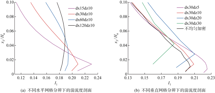
图8
不同网格分辨率方案下的湍流强度剖面
Fig.8
Turbulence intensity profiles of different mesh resolution cases
综上考虑,推荐水平网格分辨率为30 m,垂直网格分辨率为10 m,垂直网格在近地面区域适度加密.
4.3 空间差分格式对大气边界层模拟结果的影响
空间差分格式会影响N-S方程对流项的求解,为了解空间差分格式对理想大气边界层数值模拟影响,图9给出不同空间差分格式的平均风速剖面.可知,所有空间差分格式的无量纲化平均风速基本都在14.5~18.0波动,与对数律非常接近,所有相对误差基本控制在5%以内,说明空间差分格式对平均风速剖面影响不大.
图9
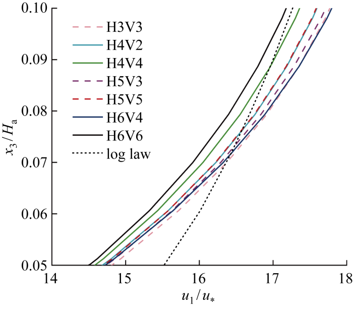
图9
不同空间差分格式方案下的平均风速剖面
Fig.9
Mean wind speed profiles of different advection differential cases
图10给出不同空间差分格式在近地面范围的湍流强度剖面.由图可知,空间差分格式在约40 m 高度范围内存在明显的差异,奇数阶差分格式较偶数阶的湍流强度更大;但在 40 m 高度以上,所有空间差分格式的湍流强度都趋于0.16.
图10
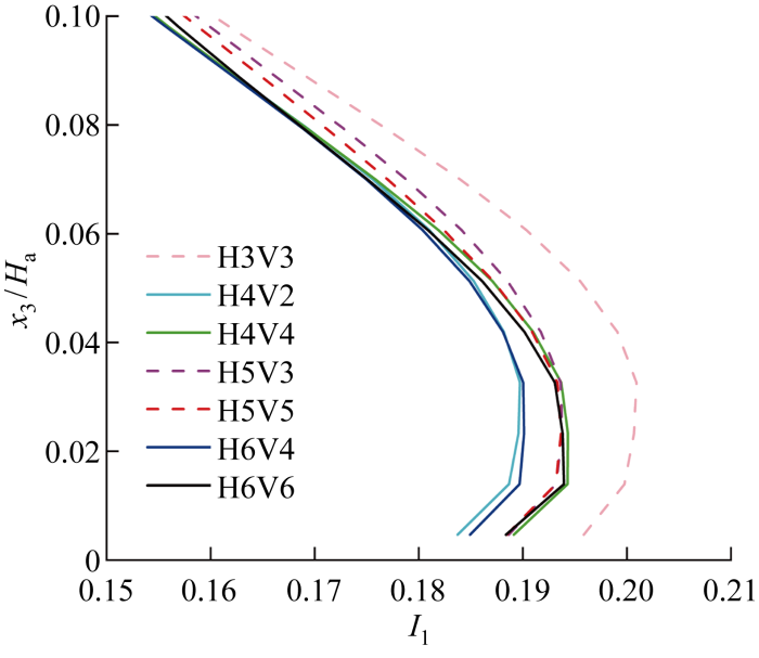
图10
不同空间差分格式方案下的湍流强度剖面
Fig.10
Turbulence intensity profiles of different advection differential cases
图11
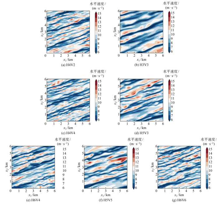
图11
在40 m高度处,不同空间差分格式方案下x-y平面水平速度的瞬时风场
Fig.11
Contours of instantaneous velocity in the x-y plane at 40 m above the surface from different advection differential cases
图12

图12
在40 m高度处,不同空间差分格式方案下的功率谱
Fig.12
Power spectrum of different advection differential cases at 40 m
表4 不同空间差分格式方案下,40 m高度处的有效网格分辨率
Tab.4
| 空间差分格式 | 40 m高度处的有效网格分辨率/Δx1 |
|---|---|
| H3V3 | 13.24 |
| H5V3 | 10.67 |
| H5V5 | 9.90 |
| H4V2 | 7.65 |
| H4V4 | 6.57 |
| H6V4 | 6.44 |
| H6V6 | 6.34 |
5 结论
利用WRF-LES模式对理想大气边界层进行模拟,结合平均风速剖面、湍流强度和功率谱等数据,分析次网格模型、网格分辨率和空间差分格式对近地面风场模拟的影响.主要结论如下:
(1) 与标准TKE模型或SMAG模型相比,NBA1次网格模型考虑了湍动能的反向级串,可更充分揭示湍流性态,更准确地模拟理想大气边界层近地面的风场特性.
(2) 结合水平网格分辨率(15、30、60和120 m)和垂直网格分辨率(5、10、20、30 m和不均匀加密)试验方案,评估其在近地面的模拟精度,建议网格纵横比设为3,水平网格分辨率采用30 m,垂直网格分辨率采用10 m;垂直网格在近地面区域适当加密可有效节约计算资源.
(3) 空间差分格式对平均风速剖面影响不大,但在WRF-LES模式下,与奇数阶差分格式相比,偶数阶差分格式,可明显改善小尺度湍流结构的再现能力,即偶数阶差分格式有效分辨率达(6~8)Δx,而奇数阶差分格式的有效分辨率为(9~13)Δx.
合适的WRF-LES参数方案可显著提高近地面风场模拟精度,有望应用于台风边界层的精细化数值模拟,提高台风风速预测精度,为防台风减灾设计提供技术参考.
参考文献
基于高精度房屋类型数据的海口市台风次生洪涝灾害损失评估
[J].
Typhoon flooding loss assessment in Haikou City based on high precision building type data
[J].
基于高塔观测的登陆台风边界层风切变指数拟合
[J].
Fitting of wind shear index in the boundary layer of landfalling typhoons based on high tower observation
[J].
Data-driven modeling of vortex-induced vibration of a long-span suspension bridge using decision tree learning and support vector regression
[J].DOI:10.1016/j.jweia.2017.10.022 URL [本文引用: 1]
Hydrodynamic experiment of the wave force acting on the superstructures of coastal bridges
[J].
利用WRF对兰州冬季大气边界层的数值模拟
[J].
The numerical simulation of the wind speed and temperature field in winter atmospheric boundary layer in Lanzhou by using WRF
[J].
基于WRF与CFD嵌套的台风下大型风力机流场作用与气动力分布
[J].
Flow field action and aerodynamic loads distribution for large-scale wind turbine under typhoon based on nesting of WRF and CFD
[J].
Coupled wind farm parameterization with a mesoscale model for simulations of an onshore wind farm
[J].DOI:10.1016/j.apenergy.2017.08.018 URL [本文引用: 1]
Time splitting methods for elastic models using forward time schemes
[J].
A class of conservative fourth-order advection schemes and impact on enhanced formal accuracy of extended-range forecasts
[J].
DOI:10.1175/2010MWR3448.1
URL
[本文引用: 1]

Starting from three Eulerian second-order nonlinear advection schemes for semi-staggered Arakawa grids B/E, advection schemes of fourth order of formal accuracy were developed. All three second-order advection schemes control the nonlinear energy cascade in case of nondivergent flow by conserving quadratic quantities. Linearization of all three schemes leads to the same second-order linear advection scheme. The second-order term of the truncation error of the linear advection scheme has a special form so that it can be eliminated by modifying the advected quantity while still preserving consistency. Tests with linear advection of a cone confirm the advantage of the fourth-order scheme. However, if a localized, large amplitude and high wavenumber pattern is present in initial conditions, the clear advantage of the fourth-order scheme disappears.
Cloud modeling tests of the ULTIMATE-MACHO scalar advection scheme
[J].
DOI:10.1175/MWR-D-10-05044.1
URL
[本文引用: 1]
Numerical diffusion can be minimized using fine grid spacing and/or higher-order numerical schemes. In this study, the authors focus on higher-order scalar advection schemes and their effects on simulated cloud fields. A monotonic multidimensional odd-order conservative advection scheme has been implemented, following the approach of Leonard. It has been tested in simulations of idealized scalar fields advected by simple prescribed motion, as well as turbulence fields; large-eddy simulations of turbulent stratocumulus clouds; and simulations of deep convective clouds. New third-, fifth-, and seventh-order schemes are compared with the second-order scheme originally used in the model. For the deep cumulus case, a high-resolution large-eddy simulation with the same domain size is used as a benchmark.
基于非线性密度流试验的平流差分方案
[J].
Tests of advection differential scheme based on non-linear density current
[J].
Numerical investigation of neutral and unstable planetary boundary layers
[J].DOI:10.1175/1520-0469(1972)029<0091:NIONAU>2.0.CO;2 URL [本文引用: 1]
A large-eddy-simulation model for the study of planetary boundary-layer turbulence
[J].DOI:10.1175/1520-0469(1984)041<2052:ALESMF>2.0.CO;2 URL [本文引用: 1]
Examining two-way grid nesting for large eddy simulation of the PBL using the WRF model
[J].
DOI:10.1175/MWR3406.1
URL
[本文引用: 1]
The performance of two-way nesting for large eddy simulation (LES) of PBL turbulence is investigated using the Weather Research and Forecasting model framework. A pair of LES-within-LES experiments are performed where a finer-grid LES covering a smaller horizontal domain is nested inside a coarser-grid LES covering a larger horizontal domain. Both LESs are driven under the same environmental conditions, allowed to interact with each other, and expected to behave the same statistically. The first experiment of the free-convective PBL reveals a mean temperature bias between the two LES domains, which generates a nonzero mean vertical velocity in the nest domain while the mean vertical velocity averaged over the outer domain remains zero. The problem occurs when the horizontal extent of the nest domain is too small to capture an adequate sample of energy-containing eddies; this problem can be alleviated using a nest domain that is at least 5 times the PBL depth in both x and y. The second experiment of the neutral PBL exposes a bias in the prediction of the surface stress between the two LES domains, which is found due to the grid dependence of the Smagorinsky-type subgrid-scale (SGS) model. A new two-part SGS model is developed to solve this problem.
Stochastic backscatter in a subgrid-scale model: Plane shear mixing layer
[J].
Implementation of a nonlinear sub-filter turbulence stress model for large-eddy simulation in the Advanced Research WRF model
[J].
DOI:10.1175/2010MWR3286.1
URL
[本文引用: 9]
Two formulations of a nonlinear turbulence subfilter-scale (SFS) stress model were implemented into the Advanced Research Weather Research and Forecasting model (ARW-WRF) version 3.0 for improved large-eddy simulation performance. The new models were evaluated against the WRF model’s standard Smagorinsky and 1.5-order turbulence kinetic energy (TKE) linear eddy-viscosity SFS stress models in simulations of geostrophically forced, neutral boundary layer flow over both flat terrain and a shallow, symmetric transverse ridge. Comparisons of simulation results with similarity profiles indicate that the nonlinear models significantly improve agreement with the expected profiles near the surface, reducing the overprediction of near-surface stress characteristic of linear eddy-viscosity models with no near-wall damping. Comparisons of simulations conducted using different mesh sizes indicate that the nonlinear model simulations at coarser resolutions agree more closely with the higher-resolution results than corresponding lower-resolution simulations using the standard WRF SFS stress models. The nonlinear models produced flows featuring a broader range of eddy sizes, with less spectral power at lower frequencies and more spectral power at higher frequencies. In simulated flow over the transverse ridge, distributions of flow separation and reversal near the surface simulated at higher resolution were likewise better depicted in coarser-resolution simulations using the nonlinear models.
Implementation and evaluation of dynamic subfilter-scale stress models for large-eddy simulation using WRF
[J].
DOI:10.1175/MWR-D-11-00037.1
URL
[本文引用: 1]
The performance of a range of simple to moderately-complex subfilter-scale (SFS) stress models implemented in the Weather Research and Forecasting (WRF) model is evaluated in large-eddy simulations of neutral atmospheric boundary layer flow over both a flat terrain and a two-dimensional symmetrical transverse ridge. Two recently developed dynamic SFS stress models, the Lagrangian-averaged scale-dependent (LASD) dynamic model and the dynamic reconstruction model (DRM), are compared with the WRF model’s existing constant-coefficient linear eddy-viscosity and (as of version 3.2) nonlinear SFS stress models to evaluate the benefits of more sophisticated and accurate, but also more computationally expensive approaches.
Improving high-resolution weather forecasts using the Weather Research and Forcasting (WRF) Model with an updated Kain-Fritsch scheme
[J].
DOI:10.1175/MWR-D-15-0005.1
URL
[本文引用: 1]
Efforts to improve the prediction accuracy of high-resolution (1–10 km) surface precipitation distribution and variability are of vital importance to local aspects of air pollution, wet deposition, and regional climate. However, precipitation biases and errors can occur at these spatial scales due to uncertainties in initial meteorological conditions and/or grid-scale cloud microphysics schemes. In particular, it is still unclear to what extent a subgrid-scale convection scheme could be modified to bring in scale awareness for improving high-resolution short-term precipitation forecasts in the WRF Model. To address these issues, the authors introduced scale-aware parameterized cloud dynamics for high-resolution forecasts by making several changes to the Kain–Fritsch (KF) convective parameterization scheme in the WRF Model. These changes include subgrid-scale cloud–radiation interactions, a dynamic adjustment time scale, impacts of cloud updraft mass fluxes on grid-scale vertical velocity, and lifting condensation level–based entrainment methodology that includes scale dependency.
RAMS and WRF sensitivity to grid spacing in large-eddy simulations of the dry convective boundary layer
[J].DOI:10.1016/j.compfluid.2015.09.009 URL [本文引用: 1]
Bridging the transition from mesoscale to microscale turbulence in numerical weather prediction models
[J].DOI:10.1007/s10546-014-9956-9 URL [本文引用: 1]
A revised scheme for the WRF surface layer formulation
[J].
DOI:10.1175/MWR-D-11-00056.1
URL
[本文引用: 1]
This study summarizes the revision performed on the surface layer formulation of the Weather Research and Forecasting (WRF) model. A first set of modifications are introduced to provide more suitable similarity functions to simulate the surface layer evolution under strong stable/unstable conditions. A second set of changes are incorporated to reduce or suppress the limits that are imposed on certain variables in order to avoid undesired effects (e.g., a lower limit in u*). The changes introduced lead to a more consistent surface layer formulation that covers the full range of atmospheric stabilities. The turbulent fluxes are more (less) efficient during the day (night) in the revised scheme and produce a sharper afternoon transition that shows the largest impacts in the planetary boundary layer meteorological variables. The most important impacts in the near-surface diagnostic variables are analyzed and compared with observations from a mesoscale network.
Comparison of convective boundary layer velocity spectra retrieved from Large-Eddy-Simulation and Weather Research and Forecasting model data
[J].
DOI:10.1175/JAMC-D-13-033.1
URL
[本文引用: 1]
As computing capabilities expand, operational and research environments are moving toward the use of finescale atmospheric numerical models. These models are attractive for users who seek an accurate description of small-scale turbulent motions. One such numerical tool is the Weather Research and Forecasting (WRF) model, which has been extensively used in synoptic-scale and mesoscale studies. As finer-resolution simulations become more desirable, it remains a question whether the model features originally designed for the simulation of larger-scale atmospheric flows will translate to adequate reproductions of small-scale motions. In this study, turbulent flow in the dry atmospheric convective boundary layer (CBL) is simulated using a conventional large-eddy-simulation (LES) code and the WRF model applied in an LES mode. The two simulation configurations use almost identical numerical grids and are initialized with the same idealized vertical profiles of wind velocity, temperature, and moisture. The respective CBL forcings are set equal and held constant. The effects of the CBL wind shear and of the varying grid spacings are investigated. Horizontal slices of velocity fields are analyzed to enable a comparison of CBL flow patterns obtained with each simulation method. Two-dimensional velocity spectra are used to characterize the planar turbulence structure. One-dimensional velocity spectra are also calculated. Results show that the WRF model tends to attribute slightly more energy to larger-scale flow structures as compared with the CBL structures reproduced by the conventional LES. Consequently, the WRF model reproduces relatively less spatial variability of the velocity fields. Spectra from the WRF model also feature narrower inertial spectral subranges and indicate enhanced damping of turbulence on small scales.
Stochastic backscatter in large-eddy simulations of boundary layers
[J].
DOI:10.1017/S0022112092002271
URL
[本文引用: 1]
The ability of a large-eddy simulation to represent the large-scale motions in the interior of a turbulent flow is well established. However, concerns remain for the behaviour close to rigid surfaces where, with the exception of low-Reynolds-number flows, the large-eddy description must be matched to some description of the flow in which all except the larger-scale ‘inactive’ motions are averaged. The performance of large-eddy simulations in this near-surface region is investigated and it is pointed out that in previous simulations the mean velocity profile in the matching region has not had a logarithmic form. A number of new simulations are conducted with the Smagorinsky (1963) subgrid model. These also show departures from the logarithmic profile and suggest that it may not be possible to eliminate the error by adjustments of the subgrid lengthscale. An obvious defect of the Smagorinsky model is its failure to represent stochastic subgrid stress variations. It is shown that inclusion of these variations leads to a marked improvement in the near-wall flow simulation. The constant of proportionality between the magnitude of the fluctuations in stress and the Smagorinsky stresses has been empirically determined to give an accurate logarithmic flow profile. This value provides an energy backscatter rate slightly larger than the dissipation rate and equal to idealized theoretical predictions (Chasnov 1991).
Subgrid-scale modelling for the large-eddy simulation of high-Reynolds-number boundary layers
[J].
DOI:10.1017/S0022112096004697
URL
[本文引用: 3]
It has been recognized that the subgrid-scale (SGS) parameterization\n \n\nrepresents \n\na critical component of a successful large-eddy simulation (LES). Commonly\n used \n\nlinear SGS models produce erroneous mean velocity profiles in LES of high-Reynolds-number boundary layer flows. Although recently proposed approaches\n \n\nto solving this \n\nproblem have resulted in significant improvements, questions about the\n true nature \n\nof the SGS problem in shear-driven high-Reynolds-number flows remain open.
Large-scale two-dimensional turbulence in the atmosphere
[J].DOI:10.1175/1520-0469(1983)040<0164:LSTDTI>2.0.CO;2 URL [本文引用: 2]
Evaluating mesoscale NWP models using kinetic energy spectra
[J].DOI:10.1175/MWR2830.1 URL [本文引用: 1]
Comparison of measured and numerically simulated turbulence statistics in a convective boundary layer over complex terrain
[J].DOI:10.1007/s10546-016-0217-y URL [本文引用: 2]
Coupled mesoscale-LES modeling of a diurnal cycle during the CWEX-13 field campaign: From weather to boundary-layer eddies
[J].DOI:10.1002/jame.v9.3 URL [本文引用: 1]
A theoretical analysis of mixing length for atmospheric models from micro to large scales
[J].
DOI:10.3389/feart.2020.582056
URL
[本文引用: 1]
A new mixing length adapted to the constraints of the hectometric-scale gray zone of turbulence for neutral and convective boundary layers is proposed. It combines a mixing length for mesoscale simulations, where the turbulence is fully subgrid and a mixing length for Large-Eddy Simulations, where the coarsest turbulent eddies are explicitly resolved. The mixing length is built for isotropic turbulence schemes, as well as schemes using the horizontal homogeneity assumption. This mixing length is tested over three boundary layer cases: a free convective case, a neutral case and a cold air outbreak case. The later combines turbulence from thermal and dynamical origins as well as presence of clouds. With this new mixing length, the turbulence scheme produces the right proportion between subgrid and resolved turbulent exchanges in Large Eddy Simulations, in the gray zone and at the mesoscale. This opens the way of using a single mixing length whatever the grid mesh of the atmospheric model, the evolution stage or the depth of the boundary layer.
